Hi! We're Elizabeth, Elizabeth and Katrina, and here's our write-up of the midlatitude eddy circulation portion of our general circulation project.
Introduction

Source: http://visibleearth.nasa.gov/view.php?id=56236
The midlatitude eddy circulation, which we can observe surrounding the pole in the satellite image above, is important for heat transport in the atmosphere. Eddies occur at higher latitudes than the Hadley Cells and as estimates in the plot below show, are responsible for most of the heat transport required by the differential heating of the Earth. Once again we used a tank experiment and atmospheric data to study these eddies. Eddies occur in the midlatitudes, where Earth's rotation is more significant. Thus, to mimic eddies in our tank experiment, we used a high rotation rate and temperature gradient. To study eddies in the atmosphere, we used atmospheric data to study the heat transport involved in the midlatitude eddies.
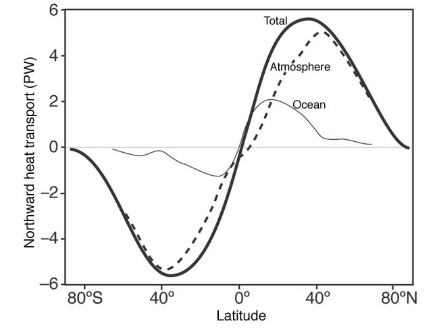
Source: "Atmosphere, Ocean, and Climate Dynamics: An Introductory Text" by John Marshall & Alan Plumb (2007).
From the figure above, detailing heat transport by latitude, heat transport is at a maximum near 40ºN and S, where eddies occur. We integrate the zonally averaged heat flux due to eddies, to find the net poleward heat flux using the following equation,

where a is the Earth’s radius, is the latitude, cp is the specific heat, g is gravity, and is the zonal average of

is the total heat flux and
is the monthly mean transport. Thus,
is the meridional heat flux due to transient eddies; using this equation we will compare its result to what the figure above predicts.
Tank Experiment
Using a high rotation rate (10 rotations per minute) to simulate the much higher Coriolis parameters at near-polar latitudes, we set up a tank experiment to observe eddy heat transport. As in the Hadley experiment, a metal bucket of ice was placed at the center of a rotating circular tank. However, due to the high rotation rate, dots placed on the surface of the water were observed to follow the shape of smaller-scale eddy currents, rather than rotating around the tank. Similarly, red and green dye placed in the tank highlighted small disturbances and rotating cells.